


Where Does the Graph Get Cut?
On a machine built from a neural accelerator, a vector DSP and a host CPU, deciding where to cut the graph costs you on every inference for the life of the product. On a Chimera core there is nothing to cut.
Summary
A network is trained in the cloud, on GPUs, in floating point. Shipping it in a product means converting it to run on the silicon in that product, and in nearly all of today's AI-enabled silicon that means a mixture of programmable cores and fixed-function accelerators. Cutting the trained graph into pieces and mapping each piece onto one of those engines is where much of an embedded AI schedule goes.
So, where does the graph get cut? On a machine assembled from a neural accelerator, a vector DSP and a host CPU, that is a real question with a real answer, and the answer costs you on every inference for the life of the product. On a Chimera core it has no answer, because there is nothing to cut. The hardware that does the multiply-accumulates and the hardware that does everything else sit inside the same processing element, take their work from the same instruction stream, and hand results to each other in registers. Everything else in this paper follows from that one arrangement.
So there is no partitioning step for you to perform. If the compiler does not already know an operator, you write it in C++ and it compiles into the same instruction stream and the same binary as everything else. Work is not assigned to processing elements either, because the array runs in lockstep and placement is settled when the binary is built.
If your part has a shared on-chip SRAM between its accelerator and its vector engine rather than a trip through DRAM, section 4 is written for you. That design removes most of the movement cost and none of the scheduling cost.
1. The question, and why you are asking it
The question we get, in one form or another, is where to cut the graph: which layers run on the NPU, which fall to the DSP beside it, what happens to the operators that fit neither, and what the tool does about all of it.
On the machine you are probably comparing Chimera against, that is the right question and it has a real answer. There is an operator allowlist. A partitioner walks your graph, matches what it can against that list, emits subgraphs, and inserts buffers and synchronization between them. What the NPU cannot take goes to the vector DSP, which means someone writes that kernel in intrinsics. What the DSP cannot take goes to the host CPU, which nobody wants and everybody eventually does. Then the partition is yours: a property of your build, tuned against one model, revisited every time the model changes.
This paper is about the first of those boundaries, between the NPU and the vector DSP. The fall to the host CPU is a third destination and a worse one, and everything said here applies to it more strongly.
Engineers who have shipped on that kind of part ask about the cut because on that part the cut decides whether the product works. It is the correct question, asked of a machine that answers it differently.
An unsupported operator on a partitioned machine runs slowly, because the engine it falls back to is one or two vector units wide, and that part you expect. The part that is rarely counted is that it also splits the graph, and the split costs more than the operator.
2. What a Chimera core is
A Chimera core is a single processor. Inside it is an array of processing elements (PEs) — 64, 256, or 1,024 of them depending on the configuration you license — and every one of those processing elements contains both of the things a neural network needs. There is a Matrix Execution Unit, the MEU, which does the multiply-accumulates that dominate a convolution or a matrix multiply. Beside it in the same processing element is a 32-bit ALU, which does the requantize, the activation, the comparisons, the address arithmetic and anything else you can write in C++. Each processing element also has a few kilobytes of its own local memory, and the array shares a larger on-chip memory behind that.
One instruction dispatcher drives the whole array, issuing a single instruction per cycle to every processing element at once. The array runs in lockstep, and both the MEU and the ALU take their work from that one stream.
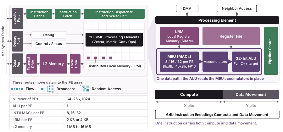
On the machines in section 1, the matrix work and the elementwise work happen in two different engines. Here they happen a few gates apart inside one processing element, driven by one instruction stream, which is why there is no boundary to schedule across and nothing to cut.
3. What a partition costs
Put those two units in separate engines and a partition costs you five things, however tightly you couple them.
The producer must materialize a whole tile. A matrix engine typically accumulates in registers that only it can address. The engine doing the requantize and activation cannot see those accumulators, so the producer writes a complete output tile somewhere both engines can reach before the consumer starts. You cannot tune that write away, because it is the boundary itself that requires it.
The handoff sets the tile size, not the algorithm. Because the consumer cannot start until a whole tile is written out, the smallest unit you can pipeline is a tile both engines agree on. Tiling stops being driven by locality and starts being driven by the interface.
The far side of the boundary does not scale with the near side. A vector DSP is one or two vector units, and its width is fixed independently of the matrix engine beside it. Scale the NPU up and the engine doing that work gets relatively narrower until it is the thing you are waiting for. A Chimera core runs the same elementwise work on one ALU per PE, so elementwise capacity scales with the array instead of being sized separately from it. There is no ratio to get wrong at design time.
The width that comes with it varies, though. At 1,024 ALUs, on a QC-Ultra, it is around ten times the INT8 lanes of a wide vector DSP; at 64, on a QC-Nano, it is comparable to one. Those are lane counts, not delivered throughput.
Two streams, two toolchains, one handshake somebody sized by hand. The engines run different instruction sets, built by different compilers, debugged with different tools. Between them is a producer-consumer relationship whose buffer depth and pipeline stage count are an engineering decision a person made.
All of it recurs, per model. A new model is a new partition, a new set of hand-written kernels for whatever the allowlist missed, and a re-tuned handshake.
4. But our engines share an SRAM
The costs above are often argued as though the boundary were a trip through DRAM. On many real parts it is not. The NPU and the vector engine share an on-chip SRAM, and the round trip people describe does not happen. If that is your part, an argument built on DRAM energy is an argument about somebody else, and you should discount everything it concludes.
The boundary between the accelerator and its vector engine gets built three ways, weakest opponent to strongest.
The DRAM boundary is the weakest case. If your accelerator hands intermediates back through external memory between fused regions you already know what that costs, and it is not the design most people are choosing now. It stays in the table below only as the reference point the other two are measured against.
The shared-SRAM boundary is the one most likely to be on your desk, and it is where the interesting argument is. Tighter still is a hardened requantize-and-activate block that reads the matrix engine's accumulators directly, and that one deserves a serious answer. All three, side by side, against the Chimera core from section 2:
| DRAM boundary | Shared on-chip SRAM | Hardened requant block | Chimera | |
|---|---|---|---|---|
| Output written to | DRAM | shared SRAM, ~6x a register access | accumulators | accumulators |
| Requantize + activation runs on | 1–2 vector units | 1–2 vector units | matrix-engine width | 1 ALU per PE, 64–1024 PEs |
| Widens as the matrix engine does | no | no | yes | yes, same silicon |
| Overlaps the next tile's MAC | only if you write the pipeline | only if you write the pipeline | yes, in hardware | yes, compiler-scheduled |
| Worst case without overlap | round trip | a full pass over the tile | n/a | one cycle |
| Op set it can apply | authored on the DSP | authored on the DSP | frozen at RTL | arbitrary C++ |
| Over the engine's budget | multi-pass | multi-pass | inexpressible | streams from L2M, one program |
| Recurs per model | yes | yes | no | no |
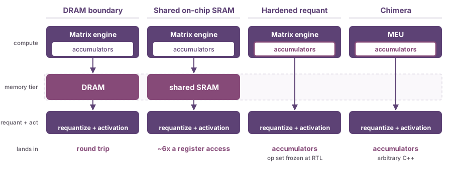
Start with the shared SRAM. The movement cost drops to something modest: a shared on-chip buffer costs roughly six times what keeping the value in the register file costs [1, 2]. That is not a headline number, and the ratio is not where the expense comes from. You pay it on every element, you cannot design it away, and it multiplies by the number of times the tensor crosses.
Some passes are algorithmic, and both machines pay them. A layer normalization needs a mean, then a variance, then the normalize; a softmax needs a maximum, then an exponent-and-sum, then a divide. Ours are no different. But our passes stay inside one kernel, in registers and local memory, while on a partitioned machine each one crosses the boundary.
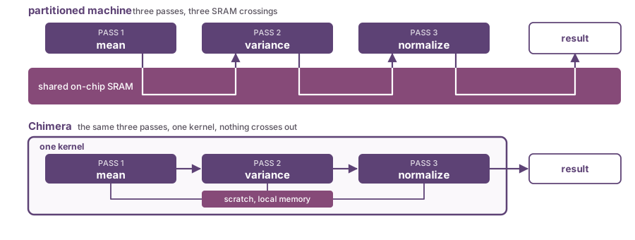
Some passes are budget-induced, and only the partitioned machine pays those. A vector engine is typically VLIW with a fixed number of issue slots per bundle, a modest vector register file, and a small local data memory. An operator that is a single pass by construction still spills when its live state exceeds that budget, and each spill is another crossing plus another traversal of the tensor.
Rather than guess at your engine's internals, look at what the work itself requires. In the residual block in section 5, a second tensor stays live across the requantize: the skip connection has to be available when the accumulator is scaled. In the activation, a 256-byte table has to stay resident alongside the tile. Both are properties of the operator, not of anyone's chip, so you can check them against your own register file and local memory.
Then the authoring cost, which is the part engineers remember: intrinsics or assembly, software pipelining by hand, double buffering against the DMA by hand, a separate toolchain, and a vectorizing compiler that frequently cannot do it for you. You do that for every operator, and you do it again for every model.
Now the hardened requantize-and-activate block, which is the strongest version of the argument against Chimera. It applies the scale, the clamp and a small set of activations directly to the accumulators. The engineering there is sound: the general engine did not keep up with the matrix engine, so the common requantize and activation went into the datapath, and freezing the operator set is what made that affordable. On movement, on overlap, and on scaling, that design matches Chimera.
It is also the only design in the table where an operator can be inexpressible. A hardened requantize-and-activate block is not a different machine; it is a fast path on the shared-SRAM machine. An operator outside its frozen set puts you back on that machine, at its width, paying materialization and whatever budget-induced passes follow. The strongest form of the argument against Chimera is strongest on the operators that already existed, and weakest on the ones you are calling to ask about.
5. You do not schedule it. The compiler does.
Here is a loop the Chimera Graph Compiler (CGC) emitted for ResNet-18. Nobody wrote it by hand.
for (int32_t ch5 = 0; ch5 < 64; ++ch5) {
  /* 210_quant */
  qVar_t<int32_t> _8 =
      nn::convTileBlockInt8<std::int32_t, 64, 3, 0, false>(ocm_tensor_5_lrm);
  qVar_t<int32_t> _9 = qBroadcast<0, std::int32_t, BroadcastAction::POP>;
  ocm_tensor_4_lrm[(ch5)] = math::max(
      cgc::qLinearAdd<31,31>(                                     /* 212_quant */
          ((qVar_t<int8_t>)math::min(
              math::max(
                  cgc::fxRoundPosInf<2>(math::fxMul<29>((_8 + _9), 7331689)), -128),
              127)),
          ocm_tensor_4_lrm[(ch5)], 0, 2146353230, 0, 1472586095, 0),
      0);
}
nn::convTileBlockInt8 is the MEU. qBroadcast pulls the bias off the broadcast bus. fxMul, fxRoundPosInf and the clamp are the ALU requantizing the accumulator. qLinearAdd folds in the skip connection. math::max against zero is the ReLU. One loop body, and nothing is materialized between any two of those steps.
The comments are the compiler's own, carried through from the node names in your ONNX file. 210_quant is the quantized convolution, 212_quant the quantized add, and the ReLU after them a third node. The last assignment in that loop finishes the convolution, performs the add and applies the ReLU: three graph nodes in one statement. The compiler answers this paper's title more convincingly than we can.
For a quantized graph, CGC fuses across what would be an engine boundary elsewhere, partitions memory, chooses tiles and schedules DMA against compute.
It also settles the numerics: fractional bits are derived from the quantization parameters and the observed ranges, so the fixed-point format is not something you specify either.
You perform no partitioning step. CGC lowers a set of ONNX operators automatically and that set grows with each release, but it bounds the automatic path, not what the machine will run. An operator outside it is named in a compile error; you write that one yourself, and it runs on the same array at the same speed in the same binary.
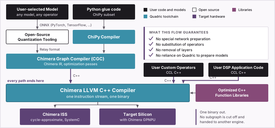
Fused does not mean always inlined: where a library kernel is the right answer the compiler emits a call to one in the same stream, and nn::softmax appears a few hundred lines further down the same generated file.
The activation is where this gets most concrete. Asked how we schedule an activation between units, the honest answer for a quantized dequantize-activation-quantize chain is that there is nothing to schedule at all:
container::NDArrayView<qVar_t<int8_t>, 256> T_qlut_lrm(cgc_core_stack_pointer, 1024);
qVar_t<std::int8_t> constants_T_qlut_lrm[] = {-123, -123, /* ... */ 117, 121, 126};
__initBuffer(T_qlut_lrm.data, constants_T_qlut_lrm, 256);
...
T_qlinear_conv2d_lrm[(ch)] = T_qlut_lrm[
    ((((qVar_t<int8_t>)math::min(
        math::max((cgc::fxRoundPosInf<2>(math::fxMul<29>((_0 + _1), 6965832)) + 66),
                  -128),
        127)) + 128))];
That is YOLOv4, and the compiler evaluated the whole chain at build time into a 256-entry table and placed it in the processing element's own local memory, so the activation costs one local read at the cheapest level of the hierarchy, inside the convolution's loop. Whether a chain becomes a table is the compiler's call, made per chain against the cost of simply computing it; where a table does not apply, the activation is evaluated in fixed point in the same stream instead.
6. Why there is nothing to schedule across
The compiler can do all of that because of where the two units sit. The MEU and the ALU are execution units on one pipeline, not engines beside each other, so there is no second program for you to write, no descriptor for you to fill in, and no other engine to wait on.
The two units also overlap:
The ALU runs in parallel with the MEU to hide the requantize and activation that follow a multiply-accumulate, which is exactly the work a partitioned machine hands to its vector engine. The compiler's instruction scheduler determines this and arranges it automatically. Where it does, the requantize and activation for one tile overlap the multiply-accumulate work for the next. Where for any reason it does not, there is nothing special to wait on: the MEU's state machine completes, the next instruction in the stream issues on the following cycle, and that is where the ALU picks up the accumulators. In one in-order stream there is no other possibility.
So the handoff costs at most one cycle, and whether you pay even that is a property of the build you can read out of the schedule rather than discover in a profile.
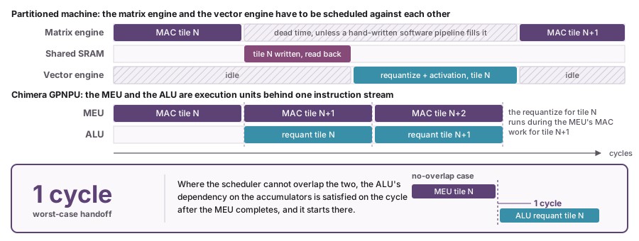
On the shared-SRAM machine, overlapping that work with the next tile's matrix work is possible and is software pipelining that you write, tune, and re-tune when the shapes change. Here it is the output of an instruction scheduler, and the worst case when the scheduler cannot manage it is a single cycle rather than a full pass over a tile.
The loop in section 5 is what this looks like in practice. The MEU call and the ALU operations that consume its result are adjacent instructions operating on the same accumulator, which is the reason the compiler has anything to interleave in the first place.
7. When you write the operator yourself
Everything so far is the supported path; the question underneath the question is usually about the other one, which is what happens when your model contains something the compiler does not already know.
Custom operators are C++. They go through the same LLVM-based compiler as the code the graph compiler generated around them, and they are linked into the same binary. The predicate stack handles their divergence the same way it does anywhere else in the array. And an operator you wrote does not create a boundary by existing, because there is no other side.
It can also consume the matrix unit's accumulators directly rather than a materialized tile, exactly as the generated convolution in section 5 does:
for(std::int32_t qCItr = 0;
    qCItr < std::min(rowsOfCToLoad, rowsOfCRemaining); qCItr++) {
  qVar_t<IntermediateType> qTempOut;
  // MEU
  qTempOut = nn::fullyConnectedTileBlock<IntermediateType, colsOfAToLoad>(qB);
  // your step, on the ALU
  if constexpr(hasLambda) {
    if constexpr(hasPostProcData) {
      qC[qCItr] = postProc(qTempOut,
                           postProcDataFlow.getData()[isPerRowData ? qCItr : 0]);
    } else {
      qC[qCItr] = postProc(qTempOut, EmptyType());
    }
  } else {
    qC[qCItr] = qTempOut;
  }
}
writeFlowC.write(qC);
postProc is a lambda the caller supplies. The step that a partitioned machine schedules as a second kernel is, here, an argument to the first, and you wrote it. An arbitrary step and a hardened one differ in exactly that.
The arithmetic in these kernels is fixed point, and the math library supplies fixed-point implementations of the transcendentals; the FP16 multiply-accumulate hardware is a synthesis-time option. On this path the fractional bits are yours to choose. For a model going through the graph compiler, the compiler derives them.
Tiling is what this path costs you today. Inside a custom kernel you size tiles against the 2 KB or 4 KB of local SRAM each PE has, and stream the rest from L2. The gap is in the authoring tools, not the architecture, and it is closing: see the appendix. For operators the graph compiler already handles, none of it is your problem in the first place.
8. Between PEs there is nothing to assign
The other half of the original question is how work gets spread across processing elements. The array executes in lockstep under a single dispatcher, so every processing element runs the same instruction: there is no per-PE work assignment to make and no per-PE schedule to balance.
Instead there is placement: the tile shape, and how a tensor reaches the array. It arrives as a Flow distributed across the array, as a Broadcast sent to every PE over a dedicated bus, or through the Random Access Unit when each PE genuinely needs an arbitrary address. Those are the three choices, the compiler makes them, and it makes them at build time. In the generated code they are visible as types:
BroadcastFlow<TensorAccessor<MinRoiDescriptor<OcmTensor<std::int8_t, 1, 1, 1, 37376>,
    AxisGroup<>, Granularity::Row, false, 1, 1, 1>>,
    OcmTensor<std::int8_t, 1, 1, 1, 37376>,
    OcmTensor<std::int8_t, 1, 1, 1, 37376>, 1>
        const_tensor_2_ocm_flow_0(const_tensor_2_ocm);
The tile shape, the granularity and the axis grouping are template parameters. They are decided when the binary is built, not when it runs, which means you can inspect them and they cannot surprise you.
9. What is still your job
Removing the partition does not remove the work; it moves it, and the two paths are not the same.
On the graph compiler path the list is short. The model has to be quantized, but not by you: the SDK quantizes an ONNX graph through sdk graph quantize, and quadric_quant does the same for a PyTorch model. What you bring is a representative calibration set, and the judgement about whether the accuracy that comes out the other side is good enough for your product. Shapes come from the model itself; only a network with a genuinely variable dimension, an LLM's sequence length being the usual one, needs you to name a maximum, and the live extent then varies under it at run time. And if you are running several models, composing that system is manual today.
On the custom-operator path, today, fixed point does become your problem: you pick the fractional bits for each intermediate in the kernel and you make sure they neither overflow nor lose the precision you needed. You also size tiles against the 2 KB or 4 KB of local SRAM each PE has. Both are authoring-tool gaps rather than architectural ones: the graph compiler already derives fixed-point formats and chooses tiles, and the custom-operator path has not yet been given the same treatment.
10. If you are coming from somewhere else
| Traditional | Chimera | Where the analogy breaks |
|---|---|---|
| Operator allowlist and a partitioner | Neither gates what runs | CGC's operator set bounds what compiles automatically, not what the array executes; outside it you write a kernel that runs at the same speed in the same binary |
| Vector DSP kernel in intrinsics | Custom operator in C++ | Same instruction stream as the graph code, and the same binary |
| Buffer and sync between subgraphs | Nothing, within a core | The consumer reads the producer's accumulators |
| Fused activation block | The ALU | Arbitrary C++; the operator set was never frozen |
| Multi-engine arbitration for two models | A second core | Spatial, so nothing arbitrates execution; they still share the memory system |
| SIMT thread blocks, occupancy, kernel launch | One stream, lockstep array | Covered in depth in our SIMT whitepaper [3]; the short version is that there is no residency to tune |
11. How to check this
Take a model you actually care about, at the batch size and sequence length you will ship, and compile it against the configuration you are considering. There is no partition report to read, because there is no partition. Read the cycle breakdown. You will find stall categories for external memory, for on-chip memory, for the array, and one named for the MEU, which is the pipeline waiting on its own accumulators. What you will not find is a category for moving a tensor to another engine, because there is no other engine.
Then take the operator you are most worried about, the one you assume you will end up hand-writing for a DSP or a CPU, and write it as a custom kernel. Do not judge it on speed at the first attempt. Judge it on whether writing it forced you to change anything else.
Appendix A: questions we get
| Question | Answer |
|---|---|
| How do I partition my graph? | There is no partition step. CGC fuses across what would be an engine boundary elsewhere. Section 5. |
| How do I schedule between the MEU and the ALU? | They are execution units behind one pipeline, and the compiler interleaves them for you. Section 6. |
| What happens to operators you do not support? | The compiler names them and stops rather than downgrading them. You write them in C++ and they run on the same array in the same stream. Section 7. |
| How do I assign work to processing elements? | The array is lockstep, so there is nothing to assign. Placement is the compiler's. Section 8. |
| What about two models at once? | Each gets its own core, its own instruction stream and its own compile-time schedule, so adding a model adds a core rather than a queue. Models that do not run at once can share one core, linked into a single binary that jumps between them at control points. Composing a multi-model system is manual today. |
| My NPU and DSP share an SRAM, so is any of this relevant? | Yes, and section 4 is written for that case specifically. |
| How do I get FP32? | You do not. There is no IEEE floating-point hardware on any unit. Inference arithmetic is fixed point, with an optional FP16 multiply-accumulate on the MEU selected at synthesis time. A layer that needs more precision can run in 32-bit fixed point on the ALU. |
| Where is the custom-operator path going? | Two ways. Quadric Kernel Language raises the level you write a kernel at, making the tiling the compiler's problem here as it already is for a graph. Beyond that, an agentic flow that writes the kernel for you. Both are in active development, not in your hands today. |
| What is still my problem? | Section 9, split by path. |
References
Y.-H. Chen, J. Emer and V. Sze, "Eyeriss: A Spatial Architecture for Energy-Efficient Dataflow for Convolutional Neural Networks", ISCA 2016, Table IV; normalized to one MAC operation, 65 nm.
S. W. Keckler, W. J. Dally, B. Khailany, M. Garland and D. Glasco, "GPUs and the Future of Parallel Computing", IEEE Micro 31(5), 2011, pp. 7–17, Table 1 and the "Locality" discussion; 40 nm.
Quadric, "Chimera™ GPNPU and SIMT: Architecture for Edge Inference", 2026, Appendix A.