


Variable-Length Prompts on Chimera™ GPNPU
A graph compiled to a fixed sequence length spends the same work on every prompt. On a Chimera GPNPU, prompt length is a value the running program carries, so one binary serves every length up to the capacity you set, and the work follows the prompt.
Summary
If you are sizing a language model for an edge product, the prompts it will see span a wide range. A spoken command is a dozen tokens, a pasted document is several thousand, and the same device serves both. Somewhere in the software stack, a decision is made about the gap between the longest prompt you provisioned for and the prompt that actually arrives. That decision sets how many binaries you build and qualify. It also sets how much of every inference is spent computing padding.
Most compiled inference stacks do not make that decision at all. A graph compiled for 1024 tokens processes 1024 positions every time it runs. If you send it fifty tokens, it computes the other 974 as padding. To serve short prompts efficiently as well as long ones, you have to build a separate binary for each length range and qualify all of them.
Quadric Chimera™ GPNPU does not work this way. It gives you one guarantee and one optimization.
The guarantee. One binary serves every prompt up to the capacity you set when you build the model. Prompt length is a value your runtime supplies when the binary runs. It is not a dimension compiled into the graph. So there is no set of per-length binaries to maintain, and nothing to re-qualify when the mix of prompt lengths changes. Capacity is a software decision, and you can change it later by rebuilding the model.
The optimization. A shorter prompt does less work. Today, key/value (KV) cache traffic and attention compute both scale with the prompt length. The projections and feed-forward layers still run at the configured length, so the compute you can save is limited. That limit exists because the software work is not finished, not because of the arithmetic. The October 2026 release removes it.
1. One binary serves every prompt length
There are two ways a system can know the prompt length. It can be fixed when the binary is compiled, with every tensor sized to it, or it can be read when the binary runs. On a GPNPU, prompt length is read at run time. The buffers are allocated once, at the configured capacity. How much of each buffer is in use is a number that the program holds and can change.
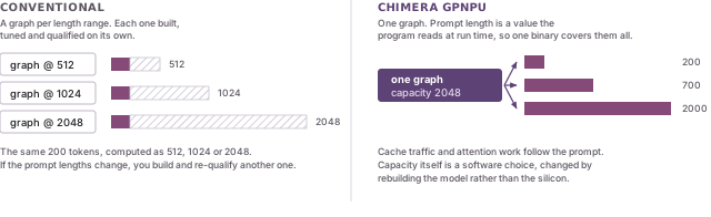
On a GPNPU, prompt length is a runtime value, so you change it by writing a register. One binary covers every length up to the capacity you configured. If the mix of prompt lengths changes after you ship, the same binary still serves it. For a product that must pass safety qualification, that matters more than any saving in compute.
KV cache traffic scales with the prompt. A prompt of two hundred tokens moves key and value data for two hundred tokens. It does not move data for the configured maximum.
Attention compute scales with the prompt as well.
Prefill is the pass that reads the whole prompt before the first output token is produced. If your runtime supplies more tokens than the configured capacity, prefill rejects the request. It does not silently drop the extra tokens. A misconfiguration therefore appears as a visible error, not as wrong output with no explanation.
2. Capacity is set when you build the model
You set capacity when you build the model. It determines the memory reserved for the KV cache and the sequence dimension of the prefill graph.
| To change | What it takes |
|---|---|
| Prompt length, within the configured capacity | Nothing. It is a runtime value |
| Maximum capacity | Rebuild the model. No hardware change, no respin |
Your GPNPU configuration sets the memory budget, which limits how much capacity is useful to build for. The capacity itself is a software choice that you can change at any point in the product's life, including after the silicon has shipped.
The KV cache itself is stored in external memory. For edge-scale models, that allocation is not the limit. While attention runs over one head, the keys and values of that head are held in on-chip L2 memory. That is where the performance comes from. So size the L2 memory to hold one full head at the longest prompt you intend to serve. Set capacity to that length, and every shorter prompt fits on chip.
You can estimate this yourself. Keys and values each take up roughly
context length x head dimension x bytes per element
so the pair together takes about 2 x context x head_dim bytes. With a head dimension of 128, a 4k context and an INT8 KV cache, that is about 1 MB per head. Switching to FP16 doubles it, so the same L2 memory holds half as many tokens. Other data also uses on-chip memory, so treat this as an estimate. We will confirm the figure for your configuration.
Because capacity is fixed at build time, you learn whether it fits in L2 when you compile. That needs the SDK, not the device, so you know before the silicon exists and long before it ships.
3. What a short prompt saves today
The question that follows is what a short prompt actually saves you today. The saving is smaller than you might expect, because not every stage of a transformer layer uses the runtime length yet.
As the prompt gets longer, three things grow at three different rates. Weight traffic does not grow at all: every token needs every weight, so the parameters stream from memory once however long the prompt is. Activation traffic, and the compute in the projections and the feed-forward layers, grow in proportion to the number of tokens. Attention compute grows quadratically with the number of tokens, because every token attends to all the tokens before it, so doubling the prompt quadruples the work.
Which of the three sets your prefill time depends on your memory bandwidth. There is a crossover prompt length. At it, the array consumes weight bytes exactly as fast as memory delivers them. Below it, memory is the limit, and all the other work finishes within the time it takes to stream the weights. Prefill then behaves like decode, the pass that produces one output token at a time: the time is spent moving parameters, not computing with them. On a QC-Ultra core with a 1024-bit interface at 1 GHz and an INT8 model, that crossover is about 128 tokens. A narrower memory interface raises it. Above it, each weight byte is reused across enough tokens that compute is the limit, and the linear stages dominate because they carry most of the arithmetic. Attention overtakes a single projection once the prompt is longer than about half that projection's width. A layer has several projections and one attention, so attention overtakes the whole layer only at around six times the hidden dimension, about 26k tokens for a dense 7B-class model. That is why attention's share stays small at the lengths most deployments configure.
Today, KV cache traffic and attention scale with the tokens you supply. The projections and the feed-forward layers could scale the same way, because each token's result depends only on that token. Today they run at the configured length regardless of the prompt. The compute saving from a short prompt is therefore limited to attention's share of the model at the configured context.
| Configured context | Ceiling on prefill compute saved |
|---|---|
| 1k tokens | ~4% |
| 2k tokens | ~7% |
| 4k tokens | ~13% |
These figures are for a dense 7B-class model. They come from counting parameters and attention operations, not from measurement on Chimera, so substitute your own model's shape. A larger configured context leaves more for a short prompt to save, because attention's share grows with the context.
The cost of attention also rises in steps, not smoothly, because the kernel processes the score grid in tiles. As a result, the shortest prompts all cost about the same. The step size depends on your configuration and is best measured on your own deployment. The projections have no such step.
Memory reservation does not shrink with a short prompt. Buffers are sized for the configured context, so a short prompt saves time and KV cache traffic but not memory. That is deliberate, because an embedded product needs a memory profile that is fixed and known before the binary ships.
All of this is a sizing problem. The waste is the gap between the configured context and the prompts you actually serve. Section 2 explains how to close it. Set capacity to match real traffic and most of that waste disappears.
4. The remaining work
Making the remaining layers scale with the prompt is work in progress. Most of it is connecting existing pieces, not inventing new ones. Both claims below can be checked.
No change to the silicon or the architecture is required. A Chimera core issues scalar, vector and matrix instructions in a single pipeline from one instruction stream. A loop bound computed at run time, and the matrix operation inside that loop, are statements in the same program, compiled for the same core. Tensors already combine a fixed allocation with a variable in-use size, so the memory footprint is known before the binary ships, and the work scales with the input.
The matrix multiplication kernel already accepts a runtime row count. The projections and the feed-forward layers are matrix multiplications, so the arithmetic itself is not the gap. The output and feed-forward-down projections add no length constraint of their own. What remains is passing the runtime length through the fused layer kernels around them, and testing the result.
| Prefill stage | Runtime length in the kernel | Used in a deployed graph |
|---|---|---|
| KV cache population | Yes | Yes |
| Attention | Yes | Yes |
| Output and feed-forward-down projections | Yes | Not yet |
| Query/key, gate and up projections | Not yet | Not yet |
| Normalization | Not yet | Not yet |
Because the linear stages carry almost all of the arithmetic, once they scale with the prompt, the prefill time scales with it too.
| Prompt, against a 1k configured context | Saved today | After this work |
|---|---|---|
| 512 tokens | ~3% | ~49% |
| 256 tokens | ~4% | ~75% |
| 128 tokens | ~4% | ~87% |
The right-hand column changes very little at a 2k or 4k configured context. The left-hand column grows with the context, as the table in section 3 shows. Below the 128-token crossover from section 3, weight streaming dominates, which is where the right-hand column stops growing. INT4 weights halve that crossover and FP16 doubles it. The figures are derived from operation counts, not measured.
We are targeting the October 2026 software release for runtime-length support in the projections and the feed-forward layers. Once those stages ship, prefill compute will scale with the tokens you supply, and the memory footprint will stay as predictable as it is today.
5. Serving longer context
In exploration.
To serve a context much longer than a full-resolution KV cache can hold, you have to store less, rather than index it differently. We are implementing the compressed sparse attention published with DeepSeek-V4 and its more heavily compressed variant. Recent tokens stay in the full-resolution KV cache. Older tokens are compressed at a fixed rate into a compact form, and the model attends to that compact form together with the recent tokens.
The persistent KV cache state for both is built. The compressor and indexer arithmetic is not yet written. Both sit alongside the existing KV cache, so the behavior described above does not change when they are added.
6. Checking this on your own model
Take a model you intend to ship and the prompt lengths it will actually see, not the maximum. Compile it once at a configured capacity that covers the longest of them. Then run that same binary at several live lengths and read the cycle counts. The KV cache transfers and the attention kernel should scale with the tokens you supplied. The projections and the feed-forward layers should not, yet. The gap between those two curves is the ceiling from section 3, measured on your own graph instead of derived from operation counts. The October 2026 release carries the runtime length through those stages. Run the same measurement on that release, and the gap closes to the savings shown in the section 4 table.
Then change the capacity and rebuild. The runtime interface does not change, and the new binary serves the same prompt lengths under a different limit. Time that rebuild, because it is the step you will repeat when your prompt lengths change.
If you want these measurements at your own GPNPU configuration before you have silicon, we can run them with you on the instruction-set simulator, and explain the KV cache interface and the attention partitioning to your engineers at the same time.
Appendix: attention measurements
Attention runs as a flash-attention kernel, tiled over keys, so the score matrix is never stored in memory. That is why attention cost scales with sequence length, and it is what both measurements below show.
Flash attention. Compared with a separate-kernel implementation at the same shape, the flash kernel takes 325,019 cycles instead of 727,546, a 2.24x reduction, with identical output. The configuration was sequence length 968, INT8, non-causal, 8 query heads over a single key/value head, head dimension 256, on 8 Chimera QC-Ultra cores. That shape comes from the Pi0.5 vision-language-action model, whose sequence length is fixed by its architecture. The comparison is between two attention implementations at one shape, and does not involve a varying length.
Attention at long sequence length. FP16 attention at sequence length 8192 fits and runs on a single QC-U core, taking 56.6M cycles and staying within 9.9e-5 of a floating-point reference, at head dimension 64. This is a capacity result, not a throughput result.
Both figures are cycle counts from our instruction-set simulator, which the Chimera Software User Guide documents at approximately 5% timing accuracy. Both measure attention alone, so multiply by attention's share of your model before drawing any conclusion about the whole network.