


Chimera™ GPNPU versus SIMT for Edge Inference
SIMT earns its generality by deferring decisions to run time. Edge inference is compiled ahead of execution, so that machinery draws power to absorb an uncertainty the workload does not contain. A Chimera core removes the machinery and keeps the generality.
Summary
Specifying AI compute for an edge product means choosing how general that engine has to be, and SIMT is the most familiar general answer: proven, programmable, and able to run whatever arrives. Outside the datacenter the question that raises is not whether the generality is worth having, but whether the mechanism that delivers it is.
A SIMT processor obtains its generality by deferring decisions to run time. Hardware forms threads and maps them onto execution resources, and a scheduler selects among resident thread contexts every cycle. The pool of those contexts is sized to absorb memory latency, and the path to main memory is cached and coalesced in hardware. A boundary separates the engine from the processor that runs the rest of the application. In a datacenter none of this is overhead, because the model, the batch size and the tenant are unknown until a request arrives, and hardware that discovers them at run time is the correct response.
Inference on an edge product is compiled ahead of execution. The model mix turns over across a product's life in market, and new models reach a deployed device as software updates, but every model arrives already compiled: its operator set fixed, its tensor extents bounded, and its batch size typically one. The machinery above continues to operate and to draw power, but the uncertainty it exists to absorb is not present in the workload.
The Chimera™ GPNPU is a general processor for inference that does not carry that machinery. The compiler maps parallelism, so no hardware repeats the work on every inference. There is one instruction stream and no pool of resident contexts. Both levels of on-chip memory are software-managed scratchpads, and there is no data cache at any level. The whole inference pipeline, including control flow and pre- and post-processing, executes in that single instruction stream without crossing a host boundary.
Whether generality survives that removal is the question, and section 1 gives two results that settle it. Convolutional networks, vision transformers, autoregressive language models from small reference models to the 30B class, and vision-language-action models for robotics all run on the same processing element array through the same toolchain. No operator in any of them has a datapath of its own. Every Quadric customer workload in production runs end to end on the array, with no part of it returning to a host processor.
1. What runs on the array
The strongest objection to removing run-time discovery hardware is that generality depends on it. A processor that does not form threads at run time, does not switch among resident contexts and does not cache an unpredicted access would be expected to execute a narrow set of operators efficiently and everything else poorly. Two results contradict that expectation.
Model coverage. The first of the two results is the range of model classes already running on one array. These figures are drawn from the several hundred networks published at app.quadric.ai/benchmarks.
| Network | Throughput | Latency | Cores |
|---|---|---|---|
| MobileNetV2 | 4,476 FPS | 0.22 ms | 1 |
| ResNet-50 | 1,379 FPS | 0.73 ms | 1 |
| ViT (Vision Transformer) | 114 FPS | 8.8 ms | 1 |
| Llama-2-15M (15M-parameter reference model) | 427 tok/s | 2.3 ms/token | 8 |
: A sample of the published benchmark set, all on QC-Ultra. Instruction-set simulator results, as published. The latency column is the reciprocal of throughput, because each of these networks runs one inference at a time.[^bench]
Three further results sit outside that table. Qwen3-8B executes end to end at 18 to 21 tokens per second on four QC-Perform cores, the mid-tier configuration with a 16 by 16 array of 256 processing elements. The Pi0.5 vision-language-action model runs end to end on one array as three dissimilar networks plus the orchestration between them: a vision transformer, a decoder language model and a flow-matching action expert. Customers have brought up autoregressive language models of their own on the same toolchain, up to the 30B class, without Quadric performing the port.
No operator in any of these networks has a datapath of its own. There is no attention unit and no convolution unit. Each network is compiled into kernels that execute on the same general array, which is the reason a class of network that did not exist when a given piece of silicon was designed can be added in software. Models already running gain from the same mechanism: a kernel-fusion change in the current release reduced Pi0.5's end-to-end cycle count by 14 percent, with no change to the silicon.
Models arrive through ONNX and PyTorch import against an operator library, and the compiler maps them onto the array: tiling, data placement and the distribution of work across processing elements are its decisions rather than yours. ChiPy® expresses pipeline-level composition in Python. An operator the library does not cover is written as a custom C++ operator, and that is the one path on which your own decomposition governs how much of the array width is used.
Pipeline coverage. Every Quadric customer workload in production executes end to end on the array. Control flow, pre-processing, post-processing and the sequencing between network stages run in the same instruction stream as the matrix arithmetic. The Scalar Element handles branching, loop management, synchronization barriers and DMA configuration, and it is part of the same core as the array it sequences. No production customer pipeline divides work between the array and an application processor.
This matters independently of model coverage, because it answers a second objection. A processor may run every network in a pipeline and still require a host for the connective material between them, in which case the boundary is still present and still has to be crossed on every inference. Here there is no such boundary to cross.
Coverage across the product family. One source description spans a range of roughly six thousand to one in throughput. It compiles from 1 TOPS on a single QC-Nano core to 108 TOPS on a QC-Ultra, 864 TOPS across a cluster, and 6,400 TOPS across 64 cores in eight chiplets. Moving between those targets is a recompilation rather than a port, because the compiler derives tiling, memory layout and data movement from the target configuration rather than requiring them to be specified per target.
Taken together, these results establish that the generality is not a consequence of run-time discovery hardware, because the processor that delivers them contains none of it.
2. What the array does not carry
That machinery is not a single overhead but five distinct mechanisms, each answering a particular unknown about the workload. Figure 1 locates them: the blocks shown hatched are the ones that resolve at run time what a compiled model has already settled.
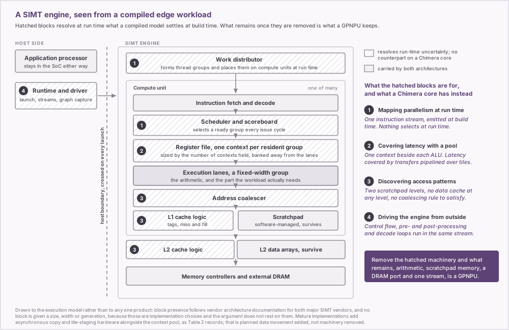
Mapping parallelism onto execution resources. An inference graph is not short of parallelism. A matrix-vector product against a 4,096-wide layer offers thousands of independent dot products, and this is true at batch size one. The question is what exploiting that parallelism costs. A SIMT processor performs the mapping at run time because in the general case it must, and therefore carries a thread abstraction, a register file multiplied by the residency factor, and selection logic that runs every cycle.
When the model is known at build time the mapping is a compile-time problem, and a processor whose compiler settles it needs no hardware to settle it again on every inference.
What follows for you is that array utilization does not depend on how many inferences are in flight; it depends on tile shape, which the compiler determines and reports at build time.
Concurrency does not reintroduce the run-time scheduling problem. A product running a vision graph, an audio front end and a decode loop simultaneously runs them on separate cores, each with its own instruction stream and its own compiled schedule. They do not contend for a shared scheduler, because the architecture contains none. A second concurrent model requires a second core rather than a place in a queue.
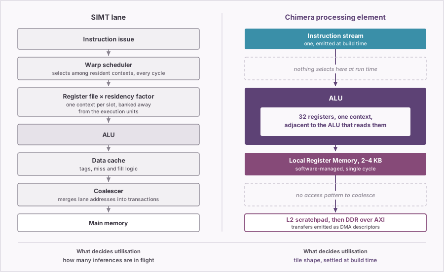
Covering memory latency. A load from external memory takes hundreds of cycles, and the arithmetic stalls unless either some other work is ready to run or the data arrived early. A SIMT engine takes the first option and a Chimera core the second. A Chimera core covers transfer latency by software pipelining over tiles: while the array computes on one tile, the next tile's input transfer and the previous tile's output transfer are both in flight. This has been the mechanism since the architecture was defined, because there was never a context pool to fall back on. Mature SIMT implementations also perform planned data movement, through asynchronous global-to-scratchpad copy and, more recently, dedicated tile-staging hardware. What they retain alongside those paths is the context pool, which serves the case where staging is insufficient or the access pattern was not known in advance. Converging on planned data movement adds a mechanism; it does not remove the one for unplanned movement.
The pool is not idle hardware. It is working correctly on a problem that a compiled inference graph does not present, and it occupies area and draws power on every cycle it is enabled. A register file sized to hold state for many resident contexts per lane is larger than one holding a single context by the number of contexts it keeps, and on the implementations for which this has been published it is a banked structure some distance from the execution units. A Chimera processing element holds one context, in 32 registers adjacent to the ALU that reads them. The corresponding exposure is that when a transfer is late there is no independent work to execute in its place, which makes the depth of the software pipeline a property of the compiled schedule and therefore something that can be inspected in the build rather than characterized after it.
Placing data. Where a tile sits and who decides where it sits are separable questions, and on the path to main memory a SIMT engine answers the second in hardware, at run time. Both levels of Chimera on-chip memory are software-managed scratchpads and neither is a cache: 2 to 4 KB of single-cycle Local Register Memory per processing element, and 1 to 16 MB of L2 memory shared across the core. There is no data cache at any level and no coalescing hardware, so there is no access-pattern rule for a kernel to satisfy in order to obtain full bandwidth.
The hardware that a SIMT processor carries here is not present by oversight, and vendor documentation states the case it serves: access patterns that are data-dependent, which a compiler cannot predict and which hardware must therefore discover at run time. That describes a graphics workload accurately. It describes an inference graph poorly. An embedding lookup fetches one row per token; mixture-of-experts routing resolves to a base address rather than a per-element gather; detection post-processing performs a bounded sort at the end. The remainder of a transformer or a convolutional network is dense arithmetic over shapes fixed before the binary exists. A compiler can place data explicitly because it knows, at build time, the bounded region each stage will access. It does not know every live address, and it does not need to: a key/value cache grows by one row per token inside an allocation whose size is fixed, and the bounded region is sufficient to emit transfers against.
Explicit placement is worth the compiler's effort because the levels are far apart in energy.
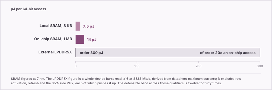
The dominant term in the external figure is the energy of reading the DRAM array itself rather than the energy of driving the package-level channel, which is why the ratio is a property of where the data resides rather than of the interface generation. Every tile the compiler keeps on chip is worth approximately that difference, and which tiles those are is visible in the build rather than being an outcome produced by a replacement policy at run time.
The host boundary. A Chimera core executes the whole inference pipeline in one instruction stream. The SoC still contains an application processor, and we provide a host API for it, but the pipeline does not span the two. On a SIMT part it does. Keeping an autoregressive decode loop off the application processor requires capturing the loop as a graph and then updating that graph's parameters on every token as the key/value cache grows. On a Chimera core the loop is ordinary control flow executed by the Scalar Element.
Which SIMT implementation. The five mechanisms described above characterize the execution model rather than any particular product. Mature implementations have added four features that reduce the cost of two of them.
| Feature | Reduces the cost of | What it takes to have it |
|---|---|---|
| Device-side kernel launch | The host boundary | Silicon support, present since an early generation |
| Graph capture and replay | The host boundary | A runtime and driver, no silicon change |
| Asynchronous global-to-scratchpad copy | Latency coverage | Silicon support, added mid-generation |
| Dedicated tile-staging hardware | Latency coverage | Silicon support, most recent of the four |
: Features added to mature SIMT implementations, and the level at which each became available.
None of the four is exotic and a current flagship has all of them. Two require silicon, one requires a runtime and a driver, and all four require the software stack that makes them usable. If you are evaluating an implementation that is not a current flagship, including one under development in-house, establish which of the four it will have, because the costs described in this section apply in proportion to how many are absent.
3. Where the difference is measurable
Different workloads exhaust different resources. At a batch size of one, the resource that runs out first is rarely arithmetic throughput, and the four cases below differ in what does run out.
Vision networks at batch size one. Vision is the case to take first, because the strongest published evidence on it is somebody else's. An independent characterization of a current edge GPU module measured five networks at batch size one: ResNet-50, YOLOv8n, MobileNetV3, an LSTM and BERT-Large. All five were found to be memory-bound in the module's highest-performance power mode. The highest throughput among them reached 1.28 TFLOP/s, under 10 percent of the platform's peak, and MobileNet reached 0.025 TFLOP/s. Energy efficiency across the five ranged from 0.6 to 22.5 GFLOP/J against a measured microbenchmark ceiling of 196 GFLOP/J on the same part.
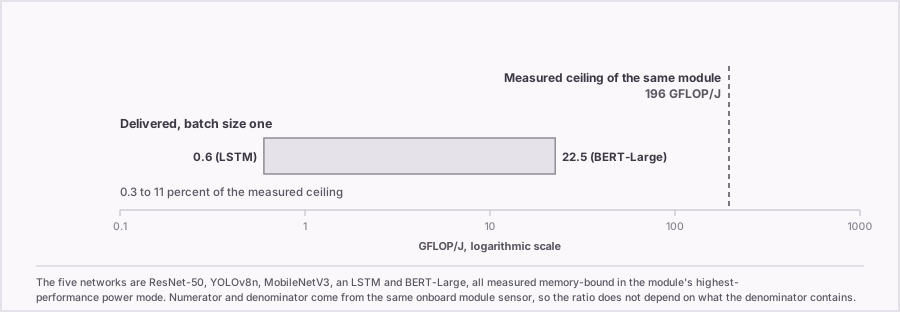
That measurement is usable in a way that a TOPS/W figure quoted between vendors is not, because its numerator and denominator come from the same onboard sensor on the same module. The ratio is therefore independent of what the denominator includes. The mechanism behind the range is the subject of section 2: these networks are memory-bound, and a context pool that exists to cover memory latency has no independent work to cover it with when one inference is in flight.
Vision transformers. Attention cost grows with sequence length, and a vision transformer presents that cost at a fixed sequence length determined by the patch count. The Chimera array can be partitioned into rectangular patches, each executing an independent matrix multiplication, which is an optional array-partitioning mode selected at implementation time and yields approximately a factor of two on production vision transformers. It partitions the array rather than specializing any part of it, and the array continues to execute the rest of the network.
A pipeline against a deadline. For a robotics pipeline the resource that runs out first is neither memory bandwidth nor the array but the number of boundary crossings permitted within the deadline. Perception, control and actuation form a sequence in which each stage depends on the one before it, and on a SIMT part each stage boundary is either a round trip to the application processor or a captured graph whose dynamic constructs are built by hand. On a Chimera core the sequence is one instruction stream, and the Pi0.5 vision-language-action model runs this way today on customer robots.
Determinism is what makes a deadline tractable on this architecture. Because there is no data cache whose contents depend on what executed previously, and no scheduler selecting among resident contexts, the same input produces the same cycle count on the data path. The published latency figures are cycle counts rather than averages over a distribution, so there is no on-chip spread to characterize and no tail to budget against. What does vary is off-chip: DRAM refresh, bank state and contention with the other masters on the AXI fabric. Licensing a core rather than buying a module makes that variance a design parameter: you select the DRAM, the arbitration policy and which masters share the fabric, and a core with a known cycle count is what lets you close that loop by analysis rather than by measurement.
Autoregressive decode. A decode step produces one token, reads every weight once and uses each weight once. Operational intensity, meaning arithmetic operations per byte moved from main memory, sits near its floor, so attainable performance is set by memory bandwidth rather than by arithmetic throughput. That holds on both architectures, and it is why beyond a certain point additional TOPS changes nothing on this workload. What differs is how much of the memory port each architecture keeps busy, and how much power is drawn by machinery that cannot raise the ceiling.
Qwen3-8B with INT4-packed weights runs at 20 to 21 tokens per second at short context lengths, falling to 18 to 19 as the context grows, because each successive step reads a larger key/value cache than the one before it. The configuration is four QC-Perform cores with 96 GB/s of DDR bandwidth between them.[^cfg] Eight billion four-bit parameters is approximately 4 GB of weight traffic per token, so 18 to 19 tokens per second corresponds to 72 to 76 GB/s of weight traffic, with the rest of the port carrying activations and the key/value cache.
The lever against that traffic is the weight format, since four-bit weights halve the traffic of eight-bit ones without reducing MAC throughput. That is INT4 today. The QD generation adds the MX formats, including four-bit floating point, and 2:4 structured sparsity, which removes the pruned weights from the fetch as well as from the multiply.
Prefill behaves differently from decode, and prompt length is a runtime value rather than a compiled-in dimension. A companion Quadric whitepaper covers prefill, prompt-length scaling and key/value cache growth.
4. Evaluating the two architectures
Peak arithmetic throughput is the figure most often quoted for both architectures, and on the workloads in section 3 it is the figure least predictive of the result. The gap between peak and delivered work on a SIMT part at batch size one is not a tuning deficit that a larger peak figure would close, which is why selecting a part by that figure does not work for these workloads.
A more useful comparison identifies the resource that runs out first on the graph in question and then asks what fraction of it each candidate converts into useful work. For autoregressive decode and for the vision networks in section 3 that resource is memory bandwidth. For a convolutional network with substantial weight reuse it is the MAC array. Both have denominators printed on every datasheet, which is not true of power.
Efficiency figures for GPU parts are frequently quoted lower than they should be. Worked from the current flagship module's published inputs, its best like-for-like figure is approximately 3.98 TOPS/W for dense INT8 over module power. Appendix B gives the arithmetic. Quadric does not place its own peak efficiency figure beside that one, because a figure for an IP core and a figure for a module measure different objects, and comparing peak against peak across mismatched denominators is the error this section describes.
Ask three questions of any efficiency figure you are shown, for either architecture: whether the arithmetic throughput is dense or sparse, at what precision it was obtained, and what the denominator contains.
5. Establishing the result on your own model
The comparison that settles it is between the two toolchains on the same workload, measured rather than inferred from datasheets. Take a model you actually care about, at the context length and batch size you intend to ship. Download the SDK from DevStudio and compile that model locally against the configuration you are considering, which returns cycle counts for your graph, with the several hundred published networks as a calibration reference. Run the same model on the other candidates and compare delivered work rather than peak throughput. That settles the question on the workload that matters to you.
No part of a Chimera core is engaged in determining what it is running, because the compiler established that before the binary existed. What remains is an array, a schedule and a memory hierarchy that can be accounted for at design time. Networks that did not exist when the silicon was designed run on it today, and those arriving after a product ships will run on it too.
Appendix A: Concept mapping for the SIMT programmer
| SIMT concept | Chimera equivalent | Where the correspondence ends |
|---|---|---|
| Thread bundle, thread block | The PE array as a whole | There are no independent thread contexts to schedule among. One instruction stream, not a pool. |
| Barrier within a block | Hardware barrier instructions | Both are hardware barriers. The scope and latency differ: single-cycle notification across cores within a cluster, rather than across threads within a block. |
| Software-managed scratchpad | Local Register Memory, 2–4 KB per element, single cycle | Closely analogous, and smaller. A second explicit level sits above it, L2 memory at 1–16 MB, also a scratchpad. |
| Global memory with a cache hierarchy | L2 memory plus DDR over AXI | Neither level is a cache. Placement is explicit and there is no data cache at any level. |
| Divergence within a bundle | Predicate stack | Paths execute as separate passes with non-participating elements disabled, as on a bundle. |
| Occupancy tuning | Tiling and placement, settled by the compiler | There is no residency to tune. A hand-written kernel defines its own access pattern instead, bounded by the Local Register Memory budget. |
| Coalescing rules | Flows and Broadcasts | Structured distribution that the compiler emits, rather than a rule an access pattern must satisfy. Flows distribute a tile across the array; Broadcasts send the same weights to every element over a dedicated bus. |
| Bank conflicts | L2 memory is multi-bank | For Flows and Broadcasts the compiler chooses placement, so bank behavior is a build-time property. Arbitrary per-element access through the Random Access Unit is where it is not. |
| Launch configuration per kernel | Compile-time array configuration | Optional modes partition the array into fixed sub-arrays or rectangular patches, settled at build time rather than per launch. They partition the array; they do not specialize it. |
| Kernel launch from the host | One binary, one instruction stream | Control code, loop management and DMA configuration execute on the Scalar Element in-stream. A host processor still exists in the SoC; the inference pipeline does not span it. |
| Per-thread arbitrary addressing | Random Access Unit | Each element requests an arbitrary L2 address. This is the path for genuinely data-dependent access, and it is more expensive than a Flow. |
: SIMT concepts and their Chimera equivalents.
Decisions that become yours. For a model imported against the operator library the compiler settles tiling and placement. When you write a kernel by hand you define its access pattern instead, and the 2–4 KB Local Register Memory budget sets how much of a working set stays local. Independently of either path, you choose and validate fixed-point representations during bring-up on the QC generation, and every tensor extent requires a bound at compile time, though not an exact size.
Practices that carry over. Tiling for locality remains the principal lever, because an access that stays on chip costs roughly a twentieth of one that does not. Data-dependent control flow still costs the sum of the paths taken. A memory-bound kernel remains memory-bound. The difference is that the compiler acts on these considerations rather than requiring you to encode them in a launch configuration.
Appendix B: Deriving the comparison figure in section 4
No TOPS/W figure is published for these modules, so the figure in section 4 is arithmetic over published inputs rather than a citation. The current flagship edge module, which contains no fixed-function neural accelerator, is specified at 1,035 dense FP4 TFLOPS against a 130 W ceiling. That figure is halved for the step from FP4 to FP8, and bridged to INT8 by the vendor's statement that FP8 and INT8 throughput are equal, which gives 517.5 INT8 TOPS over 130 W, approximately 3.98 TOPS/W, across a module that also contains its LPDDR, its regulators and its CPU cluster.
The result is a peak rather than a delivered figure, which is the distance section 4 describes.
Appendix C: Provenance and current limitations
The QC generation performs high-precision arithmetic in fixed point, so a binary point is selected and validated during bring-up. The QD generation makes FP16, bfloat16 and the MX formats native.
Every performance figure we publish, in this paper and on the benchmarks page, is produced by the Chimera instruction-set simulator rather than measured on silicon, on an isolated core with uncontended DDR. Against the HAPS FPGA prototype, simulator cycle counts for 61 vision networks land within 1.93 percent mean absolute error, with 93 percent of networks inside 5 percent. The error is a property of each model, reproducible run to run, so a published figure carries no measurement noise of its own.
Running different models on different cores is supported today, and each model retains the full benefit of the architecture. The compiler does not yet assemble such a system automatically; the composition is expressed through the host API.
We do not publish exact power or area figures without an NDA in place.
[^cfg]: Four QC-Perform cores, each with 2 MB of on-chip memory, 16 MACs per processing element and a 256-bit DDR AXI port delivering 24 GB/s, so 96 GB/s in aggregate.
[^bench]: QC-Ultra throughout, 16 MACs per processing element. ResNet-50 and ViT are published on one core at 1.7 GHz with 16 MB of L2 memory behind a 128 GB/s AXI port; the Llama row on eight cores at the same clock and port with 4 MB per core. The published MobileNetV2 entry does not state its L2 capacity, AXI width or clock.